
The impact of longevity on fiscal sustainability in South Africa - Part 2
- Oct 29, 2025
- 42 min read
CHAPTER 3
LITERATURE AND METHODOLOGY
Longevity’s impact on state finances: empirical evidence
The IMF[1] notes that the economic and fiscal effects of an aging society have been extensively studied and are generally recognized by policymakers, but the financial consequences associated with the risk that people live longer than expected—longevity risk—has received less attention. In this sense longevity can be defined as the risk that actual life spans of individuals or of whole populations[2] will exceed expectations. The IMF notes that unanticipated increases in average life span can results from:
‘Misjudging the continuing upward trend in life expectancy, introducing small forecasting errors that compound over time to become potentially significant. There is also risk of a sudden large increase in longevity because of, for example, an unanticipated medical breakthrough. Although longevity advancements increase the productive life span and welfare of millions of individuals, they also represent potential costs when they reach retirement[3].’
Longevity can broadly impact financial stability via two sources namely fiscal sustainability (e.g. as measured by deteriorating debt-to-GDP ratios) and solvency of private financial and corporate institutions (e.g. increases in their liabilities).
The Asian Development Bank Institute[4] notes that ‘(the) rapid growth of aging population can pose a serious structural challenge to fiscal sustainability. Two main channels are referred to; (1) shrinking working population who are taxpayers, and (2) increasing government expenditures for age- related programs, particularly healthcare expenditure. In other words, the government’s ability to collect tax revenue decreases due to a smaller base of taxpayers while the government expenditure, particular on healthcare spending, continuously increases ’.
Liu and Zhao (2023) links to the above research by stating that ‘The impact of population aging on finance is primarily manifested in the change in the scale and proportion of government fiscal expenditure and the increase in the level of fiscal burden in old age’. In relation to research on population again they note that there are some variabilities in findings on the impact of population aging on fiscal sustainability due to ‘different research subjects and research methods. However, in general they indicate that the academic literature on the matter shows that ‘mainstream research has concluded that population aging significantly increases the fiscal burden and leads to fiscal unsustainability’. The same authors empirically analysed the impact of population aging in100 Chinese cities between 2010 to 2019 and find that population aging significantly inhibits fiscal sustainability, to the extent that each 1% increase in population aging reduces fiscal sustainability by 0.047%. The aging of the population notably inhibits fiscal sustainability through expenditure on healthcare and fiscal expenditure on social security and employment.
Fiscal sustainability in general remains a serious challenge in the Euro Area (EA) countries, especially after the sharp rise in public debt-to-GDP ratios in the aftermath of the financial crisis of 2008. In a 2020 study, Carmen Ramos-Herrera and Sosvilla-Rivero[5] analysed data from 11 EA countries over the period 1980–2019 and finds that a higher old-dependency ratio deteriorates the cyclically adjusted government primary balance of a country, especially for countries with a relatively old population and for more indebted economies. They estimate a rise of one percentage point of the old-dependency ratio can generate a reduction of cyclically adjusted government primary balance of up to 54.5 percentage points in these countries.
Governments in particular bear a significant amount of longevity risk. The IMF identifies three main sources namely: (1) through public pension plans, (2) through social security schemes, and (3) as the “holder of last resort” of longevity risk of individuals and financial institutions. They note that ‘an unexpected increase in longevity would increase spending in public schemes, which typically provide benefits for life. If individuals run out of resources in retirement, they will need to depend on social security schemes to provide minimum standards of living’[6].
Methodology
The study uses two methods, namely time series modelling (or an extrapolation method) as well as testing South Africa’s fiscal stance against the European Commission’s S1 and S2 indicators.
Time series analysis
Anderson (2012:4) states that ‘the standard approach when assessing fiscal sustainability is an extrapolation method to project future public expenditure and revenues. The main steps are to make a decomposition of expenditures and revenues on demographic characteristics of the population in a given base year and combine this with a population forecast to generate paths for future public sector expenditures and revenues.’ He adds that and advantage of this method is that it is ‘relatively easy to apply’. However, he cautions that ‘a problem could be that it relies on an underlying path for the economic development which may not be feasible, and which disregards important adjustment mechanisms. This may bias the assessment of fiscal sustainability in an unknown direction’.
In deciding which methodology to use, the researcher is guided primarily by the type of data available. When looking at fiscal sustainability, state revenue becomes the limiting or ‘dependent’ variable against which other expenditure items are measured. We therefore first develop a workable model for state revenue, that can then be used for forecasting.
For this study we are working with time series data, which means that a time series econometric model will be utilised. The econometric modelling applied in this study is based on the Engel-Granger method[7], in which a long term (cointegrated and a priori economic theoretically correct) and short-term error correcting (“ECM”) components are combined, to provide a final (holistic) model. The error term (“equilibrium error”) from the long run model is used to link the long and short run components.
Annual time series data, from 1990 to 2023 is used for the baseline revenue modelling. This implies using least 33 observations. Once an economic meaningful and statistically significant model has been developed, it can be used for out of sample forecasting.
To determine the impact of longevity on the expenditure side of state finances, this report takes guidance from the European Commission’s (“EC”) ageing[8] and fiscal sustainability[9] reports. As far as a methodology for determining total age-related public expenditure items, the EC[10] identifies four main categories namely: health care, long-term care, education and pensions. As far as the EC’s entire age-related expenditure projection is concerned it entails four steps namely:
Making population projections;
Making exogenous macroeconomic assumptions, covering items such as the labour force (participation, employment and unemployment rates), labour productivity and the real interest rate;
Estimating the age-related expenditure items; and
Aggregating the above to provide an overall projection of age-related public expenditures.
An overview of how the different steps is combined can be seen in Figure 21.
Below is a brief discussion of the main expenditure items identified. However, it is important to note that the methodologies used by the EC are not all applicable to the South Africa economy and/or fiscal realities. For example, South Africa do not have a social security system (as defined by a mandatory publicly managed system). Also as highlighted in the first section of the report, South Africa’s demographics are (likely) more complex, notably the significant difference observed between population groups.
Figure 21: Overview of Age-Related Public Expenditures

Source: European Commission (2021), The Ageing Report, 2
Health care
In its 2021 Ageing Report[11], the EC notes that population ageing may pose a risk to the sustainability of health care financing in two ways:
Firstly, increased longevity, without an improvement in health status, leads to increased demand for services over a longer period of the lifetime, increasing total lifetime health care expenditure and overall health care spending. It is often argued that new medical technologies have been successful in saving lives from a growing number of fatal diseases but have been less successful in keeping people in good health.
Secondly, public health care is often financed by social security contributions of the working population. Ageing leads to an increase in the old age dependency ratio, meaning fewer contributors to the recipients of services. This can result in fewer people contributing to finance public health care in future, while a growing share of older people may require additional health care goods and services.
The impact of increasing longevity on health care expenditure critically depends on the health status of individuals over the additional lifetime (i.e. whether extra years are spent “in good or bad health”). Here a ‘trade off’ can develop between mortality and morbidity, e.g. in some cases mortality has decreased at the expense of increased morbidity, meaning that more years are spent with chronic illnesses. In contrast, if increasing longevity goes in line with an increasing number of healthy life years, then ageing may not necessarily translate into rising health care costs. Therefore, forecasting the health status of any population is challenging due to the difficulties associated with predicting the changes in morbidity and measuring ill-health.
Health spending is under pressure and the 2025 Budget[12] notes that ‘R28.9 billion is added to the health budget, mainly to keep about 9 300 healthcare workers in our hospitals and clinics’. Figure 22 provides the comparison between the health budget from the 2024 and 2025 budgets, with our own calculations indicating a difference (rise) of closer to R37.1 billion for the years 2025 to 2027. There is also a noticeable pickup in the trend over the Treasury’s medium-term forecast compared to the 2024 budget figures.
Table 11: Health expenditure

Source: National Treasury 2024 Budget Review, 54 https://www.treasury.gov.za/documents/national%20budget/2024/review/Chapter%205.pdf
Figure 22: Total Consolidated Health Expenditure, 2024 and 2025 Budget

Source: National Treasury, 2024 and 2025 Budget Reviews
To assess the impact of longevity this research isolates spending on health services (around 85% of the health budget), as these are the items from Treasury’s health budget, most likely to be affected by longevity risk. Population forecasts (using UN forecast) are used to calculate per capita health services spending.
Next an estimation is made of the proportion of this spending going to individuals older than 65 years.
The study assumes that government’s projections (i.e. this study’s base case forecast values) uses an unchanged stance as far as differences in population age groups and longevity is concerned[13].
The study uses earlier findings and forecasts to model longevity risk using two separate aging effects:
Structural effect: this relates to the size of the population group older than 65 years old, increasing relative to the overall population (so-called pyramid effect), and
Old age effect: this considers people literally getting older than expected.
The second (old age) effect is used to ‘reverse’ the per capita data, back to a nominal time series. The combined effect provides a longevity premium which can then be compared to the original times series.
Long-term care
For long-term care the proposed methodology considers the impact of changes in the age-structure and life expectancy of the population, on long-term care spending. It consisted of applying profiles of average long-term care expenditure per capita by age and gender to population forecasts.
The approach aims to maximise the number of factors affecting future long-term care expenditure. This may include[14]:
the future numbers of elderly people (through changes in the population projections used);
the future numbers of dependent elderly people (by making changes to the prevalence rates
of dependency);
the balance between formal and informal care provision;
the balance between home (domiciliary) care and institutional care within the formal care
system;
the costs of a unit of care.
The World Bank[15] notes that, Similar to other low- and middle-income countries (“LMICs”), the populations in sub-Saharan African countries view the family unit as the primary provider of LTC services for older family members.
The HIV/AIDS epidemic has also strained the traditional family structure in that older adults may have to care for their adult children, sick family members, or grandchildren who are orphaned or left behind by migrant parents … This presents additional challenges as older adults balance their increasingly complex health needs with caregiving responsibilities for their family members.
Financing LTC appears to be a key issue in preventing the expansion of services across the continent. Financing of programs and facilities comes from a variety of sources, including donors and non-governmental organizations (NGOs), religious organizations, and out-of-pocket payments. Even in South Africa where 74 percent of facilities are government subsidized, funds from donations and out-of-pocket payments are needed to cover the costs of care provision
South Africa is one of the few sub-Saharan African countries that has residential facilities for the elderly. Sassa[16] states that ‘if you are a senior citizen with no relatives available to take care of you in the golden age of 60 plus, there’s no need to worry. You can apply for the SASSA Old Age Grant also known as the old age pension and receive support through an old age home provided by the South African Department of Social Development (DSD).’
The SASSA website[17] notes that ‘old age homes, also called retirement homes or assisted living facilities, are special residences for seniors who require different levels of care and assistance. Depending on the home, services typically include services such as housing and meals, personal care, health monitoring, and transportation’
To qualify for admission to a government-subsidized old age home the individual must:
Be aged 60 or older
Be a South African citizen with a valid ID document
Receive the SASSA Old Age Grant or other pension fund
Need full-time frail care due to health issues (provide medical report)
Have no family or other means to be properly cared for.
However, to get aggregated data on public old age homes in South Africa is challenging. Some information is provided by the Western Cape Government[18] which notes that ‘in the Western Cape, there is a total of 300 old age homes of which, 117 are funded by the provincial DSD. For the 2020/21 financial year, R 250 million has been budgeted towards services for older persons.’
Given that the Western Cape accounts for roughly 12% of the total SA population, we can use the R250 million to estimate a total for South Africa of R2,1 billion[19] in 2020/2021.
Education
The methodology related to education spending considers the expected demographic and labour market developments, notably the ratio of students to working-age population. The hypothesis is that a reduced ratio of students to working-age population should leads to a reduction in the ratio of total education expenditure to GDP. It does not assume a general rise in the education levels but analyses the effects of expected demographic and labour market developments given the present enrolment and cost situation.
The EC[20] noted however that ‘The projections of reduced education expenditure depend on a number of variables. As no underlying trend in enrolment rates is included, wealth effects on the demand side, or investment considerations e.g. related to the Lisbon objectives, could lead to savings being even more limited. The same can happen if expenditure per student should rise relative to GDP per worker, e.g. because of smaller classes or an increase in relative wages. In addition, ‘enrolment and/or cost levels (could) increase more than what follows from the projections, because of implemented or planned legislation or other policies. This is especially relevant for enrolment in tertiary education. As education is to a large extent an investment in future human capital, many (countries) may also wish to direct any savings arising from demographic developments (rather to) increases in quality or intensity.’
Funding of education (notably tertiary education) in South Africa remains complex, notably since the ‘FeesMustFall’ campaigns and the announcement by former President Zuma at the beginning of 2018 that ‘free higher education will be provided to all new first year students from families earning less than R350 000 per year[21]’. Since then, changes have been made e.g. to change the support from a bursary scheme to a loan and partial bursary scheme[22]. The main entity offering free higher education is the National Student Financial Aid Scheme (NSFAS)[23] via fully subsidised government bursaries to qualifying students.
Given the complexities with which to determine the trade-off between demographic changes versus possible changes in legislation or other policies, this item is excluded from the analysis of this report.
Pensions (Old age grants)
The EC’s methodology includes social security and other public pensions as well as mandatory private pensions. Social security and other public pensions are broken down into two main categories:
old-age and early retirement pensions (including minimum and earnings-related pensions), with a preference to include also disability and widow’s pensions paid out to persons over the standard retirement age;
other pensions (disability, survivors’, partial pensions without any lower age limit, including minimum and earnings-related pensions).
Making this relevant to South Africa, this study will analyse likely change due to longevity in the spending on old age grants.
SASSA notes that ‘the Old Age Grant, also known as the Old Age Pension, is a South African social welfare program offering financial support to elderly citizens who are 60 years or older and have no income. Administered by SASSA Status check, this grant is available to South African citizens, refugees, and permanent residents. Eligibility is determined through a means test that evaluates the applicant’s income and assets. Once approved, recipients receive monthly payments[24]’
According to the SASSA website[25], social assistance (grants) is subject to a means test, which implies that SASSA evaluates the income and assets of the person applying to determine if these are below a stipulated amount. This currently (2024) amounts to an income of not more than R86 280 if you are single or R172 560 if married. The asset threshold is set at not more than 1 227 600 if you are single or R2 455 200 if you are married. The payments to individuals are R 2 180 per month and R2 200 for individuals older than 75 years[26].
Table 12: Social Protection Expenditure

Source: National Treasury, 2025 Budget Review https://www.treasury.gov.za/documents/national%20budget/2025/review/Chapter%205.pdf
During the 2024/25 fiscal year around 4,1 million individuals received the old age grant, and this is budgeted to rise to just below 4,5 million by 2027/28. This item represents a significant cost to the state and is also the largest (by cost[27]) of the different social grants. Old age grants cost the state R106,8 billion currently and is budgeted to increase to R131,0 billion over the next three years (that is an average rise of 7,0% per annum over the medium term) (see Tabel 12).
Like the methodology for LTC, the grant data already applies to individuals 60 years and older, and we do not need to apply a structural (‘pyramid’) effect[28]. Therefore, only an old age effect is applied.
Other assumptions
As far as this research is concerned, important macroeconomic assumptions include that:
Trends observed during the last ten (10)[29] years will continue.
Inflation is assumed to remain at 4.5% per year, that is the mid-point of the SARB’s inflation target.
GDP growth to average 2.0% per year, linked to the SARB’s potential growth calculations
The time horizon for forecasting will be 20 to 30 years.
Additional scenarios can include the assumption that a basic income grant is introduced at the food-poverty line.
S1 and S2 indicators
An important starting point for the analysis is to determine a definition for fiscal sustainability. However, this is not as straight forward as it might seem. The European Commission (EC) (2006:3)[30] notes that ‘the issue of debt or fiscal sustainability is a multifaceted one and there is no agreed definition on what a sustainable debt position is . The same commission luckily also provides a detailed definition of debt sustainability, specifically within the context of budgetary challenges posed by ageing populations, namely:
A definition of sustainability is derived from the government’s intertemporal budget constraint. It imposes that current total liabilities of the government, i.e. the current public debt and the discounted value of all future expenditure, should be covered by the discounted value of all future government revenue over an infinite horizon. In other words, the government must run sufficiently large primary surpluses in the future to cover the increasing cost of ageing and to pay off interest on outstanding debt. (European Commission, 2006:3).
This definition (related to the intertemporal budget constraint) has become known as the so-called S2 indicator. Anderson (2012:2[31]) provides an interesting angle to the discussion by noting that intertemporal budget constraint definitions do not take a stand on whether current policies are optimal, or desirable, but rather asks whether they are feasible
In addition, the EC notes that the assessment of long-term sustainability of public finances should go beyond answering the question whether current policies are sustainable or not. ‘An estimation of the size of the budgetary imbalances is also needed. This is provided by sustainability gap indicators that measure the size of a permanent budgetary adjustment’. This additional condition is known as the S1 indicator and focusses on a country reaching a pre-determined level of debt to GDP.
Since its inception these indicators have also been revised and a 2023 report[32] by the EC notes that ‘(t)he S2 indicator measures the fiscal effort needed to stabilise public debt over the long term. The revised S1 indicator measures the fiscal effort required to bring the government debt-to-GDP ratio to 60% in 2070[33], hence capturing vulnerabilities due to high debt levels. The methodological approach differs from the Fiscal Sustainability Report 2021, which determined long-term fiscal risks based on the S2 indicator and the DSA results. The revised S1 indicator provides a better long-term complement to the S2 indicator, as based on a similar time horizon.’
The EC’s uses the following equation to forecast the evolution of the debt-to-GDP ratio:

(Equation 1)
Where:

Related to the impact of ageing on the S2 indicator, it is explained that (ceteris paribus) the higher the projected cost of ageing, the more difficult it is to fulfil the intertemporal budget constraint, as higher revenue – in present terms – is required to cover these costs, in addition to the other non-interest expenditure and debt service (European Commission, 2023:71)[34]
In practice, various types of fiscal balances exist, which according to the IMF[35], often ‘relate to special issues or circumstances and are only partial approaches and indicators for assessing complex situations. Some of the diffident types include:
Current fiscal balance: this represents the difference between current revenue and current expenditure. It provides a measure of the government's contribution to national savings. When positive, it suggests that the government can at least finance consumption from its own revenue.
Primary balance: this balance excludes interest payments from expenditure. It can be said to provide an indicator of current fiscal effort, since interest payments are predetermined by the size of previous deficits. For countries with a large outstanding public debt relative to GDP, achieving a primary surplus is normally viewed as important, being usually necessary (though not sufficient) for a reduction in the debt/GDP ratio.
Cyclically adjusted or structural balances[36]: this item seek to provide a measure of the fiscal position that is net of the impact of macroeconomic developments on the budget. This approach takes account of the fact that, over the course of the business cycle, revenues are likely to be lower (and such expenditure as unemployment insurance benefits higher) at the trough of the cycle. Thus, a higher fiscal deficit cannot always be attributed to a loosening of the fiscal stance but may simply reflect that the economy is moving into a trough.
According to the National Treasury, ‘the government's fiscal balance before accounting for interest payments on its outstanding debt. It is calculated as the difference between total government revenues and total non-interest expenditures. A positive primary balance indicates that the government’s revenues exceed its non-interest spending, while a negative primary balance suggests a shortfall[37]’.
As far as its relevance to fiscal studies Bond Economics[38] notes that ‘the standard working assumption is that the primary balance is the result of fiscal policymakers, and that they do not wish to depart from this set policy. For example, they do not want to be forced to raise or lower taxes, as that has political consequences. The same holds true for programme spending. The usual interpretation of holding the trajectory of the primary balance fixed is to see whether the current fiscal policy settings are "sustainable"’ However, the same source also cautions that ‘the basic problem is that it makes very little sense for fiscal policymakers to care about the primary balance. Taxes are not imposed in the form of absolute levels; they are almost always imposed as percentages of nominal incomes and activity (e.g., income and sales taxes). As such, the tax component of the primary balance will shift based on the economic cycle, even if policy settings are unchanged…The net result is that the primary budget balance moves in a counter-cyclical fashion with the business cycle (deficits rise during recessions)’.
In applying the EC’s methodology to this research, the development of the primary budget balance will be analysed to determine its relevance to the overall debt trajectory (S2) and to quantify what it should be to bring the debt-to-GDP ratio down to 70% of GDP[39] by 2055 (S1). Factors impacting longevity will be included via the adjusted expenditure figures, as discussed in the previous section.
CHAPTER 4
ANALYSIS
As explained in Chapter 3, the analysis uses two methods, namely time series modelling (or an extrapolation method) as well as testing South Africa’s fiscal stance against the European Commission’s S1 and S2 indicators.
Time Series Analysis
At its core, fiscal analysis boils down to two items namely government revenue and expenditure. When looking at fiscal sustainability, state revenue becomes the limiting or ‘dependent’ variable against which expenditure items are measured. This section therefore first presents a workable model for state revenue, that is used for forecasting.
From here a base scenario is created in which existing expenditure trends (evident during the past 5 to 10 years), are extrapolated and compared to the estimated development in revenue (as obtained from the econometric model).
The next step it to apply shocks to the base scenario, notably by changing expenditure items that are likely to be impacted most by longevity risks. Additionally, the implementation of a BIG (Basic Income Grant), is also analysed.
Government revenue model and forecast
Econometric model
A time series can be defined[40] as a set of observations on the values that a variable takes at different times. Such data is usually collected at regular time intervals, such as daily (e.g. stock prices, weather), monthly (e.g. inflation, money supply), quarterly (e.g. GDP), annually (e.g. government budgets) or even at longer time intervals.
Although time series analysis is used heavily in econometric studies, it does present specific problems, notably the assumption that underlying time series are stationary. In short, stationarity can be defined as a time series for which the mean and variance do not vary systematically over time.
However, by using cointegration techniques, as proposed by the econometricians Clive Granger and Robert Engle, or generally referred to as the ‘Engel-Granger’[41] type analysis, time series that are non-stationary can be shown to share the same common trend so that regression analysis will be meaningful (i.e., not spurious). They are thus said to be cointegrated. Economically speaking, variables will be cointegrated if they have a long-term, or equilibrium, relationship between them.[42] Short run disequilibrium is likely to still exist, but this is corrected by the error correction mechanism (“ECM”),[43] as also proposed by the Engel-Granger method.
The econometric modelling used for government revenue in this Report is based on the Engel-Granger method, in which a long term (cointegrated and a priori economic theoretically correct) and short-term error correcting (“ECM”) components are combined, to provide a final (holistic) model. The error term (equilibrium error) from the long run model is used to link the long and short run components. Therefore, this term (i.e. its coefficient and statistical properties) becomes very important in the ECM, as also discussed in more detail below.
Annual time series data, from 1990 to 2023 is used for the baseline revenue modelling. This implies using 33 observations. All data was sourced from the South African Reserve Bank, National Treasury and Statistics South Africa. Because budget data is usually reported in fiscal years, the researcher must take cognisance of other economic variables provided in calendar years, which could impact the comparability of the different datasets. Fortunately, the SARB also provides calendar year values for most of the major state finance line items. The revenue model presented here is therefore run on annual (calendar) year data[44].
The long run component of the modelling process is done to obtain a cointegrated, long-term trend, or equilibrium relationship between variables. In this sense one wants to rather use fewer variables, that are likely to have theoretically sound economic impacts on the dependent variable. For this purpose, GDP and household disposable income was used and it was confirmed that there does exist a cointegrating relationship between the long run variables (see details in Addendum 1).
The short run component, also known as the error correction mechanism (“ECM”), is defined as the part of the model that corrects for disequilibrium. Variables included in the ECM included household disposable income, the prime interest rate, money supply (“M3”) and inflation. In addition to this the long run component are included (as required) via the residual variable from the long run equation (i.e. ‘Res_Rev’). All variables were differenced appropriately for stationarity and the relevant diagnostic and stability tests confirmed. The detailed specifications and estimated results are provided at the end of this chapter in Addendum 1
In general, the model indicates a good fit as the modelled values closely follows the trend of the actual values (see Figure 23). Some discrepancies are evident towards the later part (around 2020). However, these are to both the upper and lower side, meaning we do not have a specific direction of bias in the model. The large fluctuations in the data itself during the Covid-19 period (2020-2021) likely further complicates the model’s ability to trace the actual values.
Figure 23: Revenue Model: Actual and Fitted Values (Real, R millions)

Source: Own calculation
Revenue forecast
Out of sample forecasting is performed next, for the period 2024 to 2055 – that is over a period of three decades. The assumptions for the explanatory variables are as follows:
CPI and Inflation: increase of 4.5% per year (as per the mid-point of the SARB’s inflation target)
GDP: Real increase of 2.0%[45] per year
RYD: Real increase of 1,2% per year (average of last 10 years)
RM3: Real increase of 2,1% per year (average of last 10 years)
Prime: Decline from its current value to 9.5% per year over the next four years (until 20207), and then remain fixed at that value (9,5 based on the average of the last 10 years)
Base scenario
To make the results from the revenue model comparable to expenditure, the real values are deflated using the CPI. This indicates a continued upwards trend in (nominal) government revenue. Over the short term the modelled annual growth in revenue picks up from 2.3% in 2023 (actual) to 6.9% and 7.7% during 2024 and 2025 respectively. Over the long term (2030 and beyond) the growth rate settles on around 7.1% per year. This compares very well to the historic average growth of 7.2% per year recorded by this item during the last decade.
As explained in the methodology section, government expenditure is forecasted using an extrapolation (moving averages) method. To obtain the likely long-term trend in expenditure, it is increased by 6,9%[46] per year – equal to the average rise in this item during the last decade.
Figure 24: Revenue Model: Actual and Forecasted (@1,5% and 2% GDP growth)
(Real, R millions)

Source: Own calculation
Figure 25: Base Scenario: Long term Estimates for Revenue and Expenditure
(Nominal, R millions)

Source: SARB data, Own calculations and forecasts
Evident from the comparison of the two long term forecasts, is that expenditure continue to outperform revenue over the forecast period. Reasons for this include that, government is currently running a budget deficit, meaning that expenditure starts from a higher value. Also, despite the higher projected growth rate in revenue (7.1% from 2030 onwards) compared to 6.9% average for expenditure, revenue is struggling to make inroads into expenditure, even over the 30-year time horizon.
Another way of looking at this is to calculate the projected budget balance, which indicates a gradual decline from a deficit 6,0% of GDP in 2023 to around -5.8% in 2030 and only dipping below -5.5% of GDP from 2050 onwards (see Figure 26).
This means that under the base scenario the budget deficit is expected to remain negative, albeit declining, over the forecast horizon.
In addition, this means that state debt will continue to climb to fund the annual deficits. Given a rise of 2.0% per year in GDP, debt is expected to continue rising but also to stabilise just below 90% of GDP around the middle of the 2040’s.
However, if the economy only manages to record growth of 1.5%, the debt level is expected to continue accelerating, reaching 90% of GDP in roughly a decade (i.e. around 2034).
Figure 26: Budget Balance as % of GDP (@1,5% and 2% GDP growth)

Source: SARB data, Own calculations and forecasts
Figure 27: Gross Debt to GDP (@1,5% and 2% GDP growth)

Source: SARB data, Own calculations and forecasts
Evident from the above is that in order for debt levels to remain below 90% of GDP[47], the economy will have to grow by a level of at least 2,0% per year[48]. Any value less than this will mean a continued upwards trend, i.e. to clearly unsustainable debt levels.
However, the aim of this section is to establish a base scenario on which further analysis can be performed. For this reason, it the (more optimistic) 2,0% per year GDP assumption will be applied during the remaining of this Section.
Longevity impact scenario
The aim of this section is to quantify and analyse the impact of longevity on a selection of government expenditure items, as identified in the methodology. The items will be quantified individually after which the combined impact will be analysed against the forecast results from the base scenario model.
Health care
The impact on healthcare is calculated by only using health services related spending (around 85% of the total health budget) and using population forecasts to calculate per capita figures. Two separate aging effects are then analysed namely a structural effect (relative size of the population older than 65 to the total population) and an old age effect (people living longer than expected).
Initially health services spending is calculated by using 84.8% of total health expenditure up to 2027 (for which National Treasury data is available), after which it is forecasted by using the 10-year average ratio of this item to total expenditure.
Structural effect
Per capita health services expenditure is calculated , and from there the proportion of this relevant to the elderly (65+) is calculated using a fixed ratio of 6,5% of the population (i.e. the ratio where this age group was at 2024). A second scenario uses an increasing ration (i.e. individuals over 65 years old increasing from 6.5% to 11.2% of the total population). Figure 4.6 provides the results of the two scenarios.
Figure 28: Per Capita Spending by Elderly (65+) on Health Services (Base and Shocked Scenario)

Source: Own calculations
Old age effect:
In addition, a longevity effect(i.e. the risk that life expectancy is underestimated) need to be added, which is done by applying an aging coefficient (around 0.5 percent per year) to only the population older than 65 years[49]. In brief this increases the size of the 65+ population group in 2055 by around 1.4 million individuals. The ‘new’ total population is then calculated by replacing the old age group with the new numbers. See Figure 29 for the impact of this adjustment. This adjusted population data is used to re-calculate the nominal rand values.
Figure 29: Total Population (Base and Alternative Scenario)
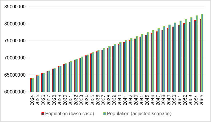
Source: Own calculations
Total healthcare effect
The results indicates that the gap (difference) between the base and shocked scenario will continue to increase over the forecast period, reaching and amount of R110,0 billion in 2055.
Figure 30: Health Services (Base and Shocked Scenario)

Source: Own calculations
Another way to look at this is to compare the gap to total government expenditure, which indicates a shock starting at less than 0.1% of total expenditure around 2030 but rising to around 0.6% of total expenditure in 2055 (see Figure 31).
Figure 31: Health Shock to Expenditure

Source: Own calculations
Long-term care
For long-term care the analysis focus on the impact of changes in life expectancy of the population. Specifically, how these factors are likely to impact the cost of providing public old age homes by the South African Department of Social Development (“DSD”).
As mentioned in the methodology section, it proved difficult to find aggregated data on public old age homes. Some data from the Western Cape Government indicated that in 2020/21 this province spent R250 million on services for older persons.
Using this as a benchmark we estimate a spending for South Africa of around R2,1[50] billion during the same year.
As base scenario this amount is inflated (using an annual inflation rate of 4.5 % per year). This takes LTC spending from around R2.4 billion in 2024 to R9.4 billion in 2055.
To determine the likely impact of longevity on these figures, a shocked scenario is then developed. As the data already applies to individuals 60 years and older, we do not need to apply a structural (‘pyramid’) effect[51]. Therefore, only an old age effect is applied.
The resultsare presented in Figure 32, which indicates a difference between the base and shocked scenario reaching R500 million in 2040 and further increasing to around R1.5 billion by 2055.
Figure 32: Long term care (“LTC”) Costs (Base and Shocked Scenario)

Source: Own calculations
Compared to total government expenditure, the LTC shock is fairly small[52], rising to around only a 10th of a percent by 2055.
Figure 33: LTC Shock to Expenditure

Source: Own calculations
Pensions (Old age grants)
The analysis focus on how changes in life expectancy of the population could impact pension payments. Specifically, how this is likely to affect the cost of social assistance payments (so called old age grants).
Like previous sections, a base and shocked scenario is developed. The base scenario uses data from the National Treasury up to 2027/28 after which the item is expected to increase equal to the 10-year average (that is 8.6% per year for old age grants).
The shocked scenario uses this same base data and forecasts but applies an old age coefficient to capture the impact of people in general living longer than expected.
The results are presented in Figure 34 which indicates a difference between the base and shocked scenario reaching R30 billion in 2040 and further increasing to around R195 billion by 2055.
Figure 34: Pension Costs (Base and Shocked Scenario)

Source: Own calculations
The results indicate a relatively large gap averaging 0,5% of total expenditure over the forecast period. Annual values of more than 1% of total expenditure is reached from 2050 onwards (see Figure 35).
Figure 35: Pension Shock to Expenditure

Source: Own calculations
Combined (Health, LTC and pensions)
By adding the three items (Health, LTC and pension), the total impact is derived. In rand value the impact (shock) on total government expenditure is expected to increase over the forecast period, reaching around R40 billion in 2040, and increasing to over R300 billion by 2055.
In percentage terms, this is equal to an average rise of around 0,8% of expenditure over the period, with annual values reaching 1,0% in 2040 and peaking at 1,7% in 2055 (see Figure 36).
Figure 36: Total Shock to Expenditure (R value and %)

Source: Own calculations
Figures 37 shows the relative contributions of the three items to the total shock, which clearly indicates the dominant impact of old age grants, followed by the health services effect.
Figure 37: Total Shock to Expenditure (Components)

Source: Own calculations
Impact on fiscus
The last part of this section is to consider the impact of the shocked expenditure values on South Africa’s overall fiscal stance. This is done by comparing it to the modelled revenue values and base scenario developed in Section Four. Note that the base scenario using 2% GDP growth[53] is used for comparison.
The base scenario indicated that the budget deficit is expected to peak at 5.8% of GDP around the mid-2030s,after which it will gradually decline to around 5,4% by the end of the forecast period. In contrast to this, the shocked scenario does not see a peak, but instead for the deficit to continue increasing (worsening) over the forecast period, to reach just below 6% of GDP in 2055 (see Figure 38)
Figure 38: Budget Balance as % of GDP (Base and Shock)

Source: SARB data, Own calculations and forecasts
In addition, this means that state debt will continue to climb to fund the annual deficits. In the base scenario debt is expected to stabilise just below 90% of GDP around the middle of the 2040’s. Again, in contrast the shocked scenario does not see a peak, but indicates a continual rise, breaking the 90% level around mid-2040’s and climbing to 93% of GDP by 2055. On average this will mean a higher debt to GDP ratio of around 1.8 percentage points over the forecast period.
Figure 39: Gross Debt to GDP (Base and Shock)

Source: SARB data, Own calculations and forecasts
Impact of longevity and Basic Income Grant (“BIG”)
As a last part of this section, the aim is to analyse the impact of a possible Basic Income Grant (“BIG”) being implemented. The assumption here is that the existing (temporary) Covid-19 SRD grant be transferred to a basic income grant. The 2025 Budget indicates that around 8,3 million individuals are receiving the SRD at a cost of R35,5 billion to the state.
We assume that the BIG will be implemented at the food poverty line, which is R796 per month (“StatsSA[54]”). To provide this to 8,3 million individuals will cost the state around R79,3 billion per year. That is roughly double the amount of the SRD.
In addition, we assume that part of the individuals receiving the grant could in future also need old age assistance, thus the values are also adjusted for and ageing coefficient. The BIG is assumed to be implemented in 2025.
The results indicate that the budget deficit is likely to increase by around 1 percentage points, compared to the shocked scenario. For 2025 this is equal to a deficit of 7,0% of GDP, which is expected to gradually decline to around 6,6% by the end of the forecast period.
Figure 40: Budget Balance as % of GDP (Base, Shock and BIG)

Source: SARB data, Own calculations and forecasts
As can be expected this will push the debt to GDP ratio up even further, now breaking 90% by 2033 and 100% in 2044. This also adds a significant increase over the shocked scenario, of an average of 8,1 percentage points higher over the forecast period.
Figure 41: Gross Debt to GDP (Base, Shock and BIG)

Source: SARB data, Own calculations and forecasts
S1 and S2 indicators
The S2 indicator measures the fiscal effort needed to stabilise public debt over the long term while the S1 indicator measures the fiscal effort required to bring the government debt-to-GDP ratio to a measurable target at a specific date in future. Both these indicators have a strong focus on the development of the primary budget balance, that is the difference between total revenue and non-interest expenditure, and how this in turn affects the trajectory of government debt levels.
This section first looks at general trends in South Africa’s budget and primary budget balances after which the two indicators are analysed. This builds on the work of Section Four, in as far as the longevity impact on expenditure has already been developed and can thus be further utilised here.
Overview of fiscal balances
An overview of the post-1990 trends in South Africa’s fiscal balances, indicate three distinct periods:
Prior to 1994: Worsening of fiscal stance as the state ran continued larger deficits, reaching -7.5% of GDP in 1993.
1994 to pre 2008/09 GFC: The improved economic climate re South Africa, after 1994 is evident as the fiscal deficits got smaller, to a point where surpluses were recorded during 2005 and 2006. The primary balance improved significantly and recorded surpluses, averaging around 3% of GDP, during the period 1995 to 2008. Also noticeable during this period is the narrowing in the gap between the fiscal budget and primary balances (In figure 4.19 this is evident from the light blue and orange lines converging during the period).
Post 2008/09 GFC: There is a clear switch in sentiments during (and after) the 2008/09 Global Financial Crisis as a large fiscal deficit of -4.7% is recorded in 2009, while the primary deficit records -2.6% of GDP. Both these indicators remain in negative territory (deficits) until 2019, during which a widening (divergence) between the two are again observed (likely as debt starts to increase, driving up debt-service costs). The further severe impact of the Covid-19 crisis is evident in large deficits recorded during 2020-21.
Figure 42: South Africa’s Budget and Primary Balances, 1990 to 2022

Source: World Bank
Comparing developments in the primary balance to government debt, shows a decline in debt levels between 2000 to 2007 (that is when large primary surpluses were run). 2008 again indicates an inflection point, that is a sharp and sudden reversal in trends as debt starts to climb post the 2008/09 GFC, while the primary balance falls and records deficits for the remainder of the period (up to 2022) (see Figure 43).
As far as more recent developments the Treasury seems to be committed to focus on establishing and maintaining a primary surplus. The 2025 Budget Review[55] notes that ‘government projects a main budget primary surplus of 0.5 per cent of GDP, which will increase to 0.9 per cent in 2025/26’ and that this ‘will achieve a longstanding ambition to stabilise debt next year through the strengthening primary surplus. The fiscal strategy will continue to manage fiscal risks, support essential services and encourage economic growth.’
Figure 43: Primary Balance and Debt, 2000 to 2022

Source: World Bank
It is evident that the state is also looking for potential fiscal anchors ‘to support responsible borrowing and spending. In 2025/26, the debt stabilising main budget primary surplus will serve as the fiscal anchor, with larger primary surpluses planned for the remainder of the decade to reduce debt as a proportion of GDP[56]’.
However, worrying are statements[57] made after the 2025 budget by the Minister of Finance regarding a change in the budget’s focus from ‘spending cuts to higher taxes’, as these could undermine the proposed fiscal anchors as well as outlook of the primary balance. There also remain some uncertainty over some budgeted proposals (notably the implementation of the proposed VAT hike(s)).
Table 13: 2025 Budget: Main Budget Framework

Source: 2025 Budget Review, 31
S2 indicator
The S2 indicator measures the fiscal effort needed to stabilise public debt over the long term. In this case we use equation 1 (see Chapter Three) to estimate the future trend of debt. The starting point is to forecast data for the explanatory variables, after which Dt (the debt-to-GDP ratio) is calculated.
The primary budget balance plays a critical role in these calculations and is obtained as the difference between revenue and non-interest expenditure. To obtain non-interest expenditure, we use the (shocked) expenditure values (obtained earlier in this Chapter[58]) from which debt service costs are subtracted. This is then expressed as percentage of GDP, using the nominal GDP values. Over the medium term (2026 to 2028) National Treasury’s projections[59] from the 2025 budget is used (see the last row in Table 4.1 above). To forecast the values, the 10-year average (i.e. 2019 – 2028) is used, which equals a value of -0.5% to GDP.
To limit the number of ‘moving parts’ the forecasts for the nominal GDP and nominal interest rates (Repo) are kept pegged at their 2024 values.
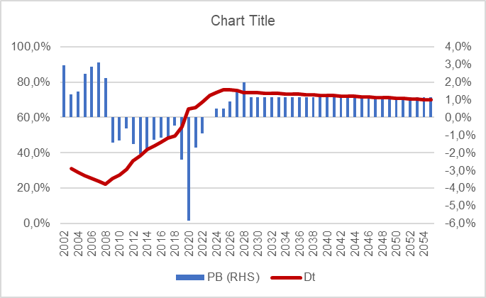
Figure 44: Primary Balance and Debt Forecast (S2), 2002 to 2055

Source: National Treasury and own calculations
Using the above, the debt trajectory is expected to continue increasing and breach 90% of GDP by 2038 and 100% around mid-2040s.
Further interesting conclusions include that the debt level continues to rise as long as the primacy balance remains negative, albeit by a small margin.
S1 indicator
As explained previously, the S1 indicator will be modified to measures the fiscal effort required to bring South Africa’s government debt-to-GDP ratio to 70% by 2055.
From the S2 scenario we know that any negative value will not be sufficient to stabilise the debt trajectory. Therefore, it is evident that the value for PB needs to be some positive value. By testing different forecast scenario’s, it was determined that a primary surplus of at least 1.15% of GDP needs to be maintained throughout the forecast period to bring the debt level down to 70% of GDP by 2055.
This compares well to National Treasury’s statement (see Section Four) that the ‘primary surplus will increase to 0.9 per cent in 2025/26’ and that this ‘will achieve a longstanding ambition to stabilise debt’. Albeit that this research indicates that an even higher surplus will be required to actually drive down the debt level.
Figure 45: Primary Balance and Debt, S1 Adjusted
Source: Own calculations
S1 and S2 criteria
The European Commission provides various criteria against which to compare the results. This includes a decision tree (see Figure 46) and threshold levels for the different indicators (see Table 47).
If we start with the S2 indicator as calculated for South Africa, the debt level in 2032 is expected to be 80,4%, placing the country in the medium (‘between 60% and 90% of GDP’) risk category. However as far as the debt trajectory is concerned, it is evident that it should ‘still increase at end of projection’ placing the country in the high category. According to the decision tree (Figure 46), at least one high risk item is sufficient to conclude that South Africa will fall in the high-risk category as far as overall (i.e. S2) debt sustainability is concerned.
Figure 46: Decision Tree for Assessment of Fiscal Sustainability Risks

Source: European Commission[60], p183
As far as S1 is concerned the criteria state that ‘the risk classification derived from S1 depends on the amount of fiscal consolidation needed to reduce debt to 60% of GDP over the medium term. When this requires a large effort of more than 2.5% of GDP on top of the baseline assumptions, this identifies a high risk. When no additional effort is needed as debt is already projected to stand below 60% of GDP, corresponding to a negative S1, the risk is low. For intermediate values of S1, the risk is medium[61]’.
Figure 47: Debt Sustainability Thresholds

Source: European Commission[62], p185
Important to note is that, in this research both the forecast horizon (2055 rather than2070) and point target (70% of GDP instead of 60% of GDP) differs from that used by the EC, which complicates then comparison
However, using the required correction value of 1.15% of GDP as calculated above, this will put South Africa in the ‘intermediate’ or ‘medium risk’ category as far as the S1 indicator is concerned.
Combining the S2 and S1 indicator puts South Africa in a ‘high/medium’ overall risk category.
CHAPTER 5
CONCLUSIONS
The aim of this study is to assess the impact of longevity (i.e. people living longer than expected) on fiscal sustainability in South Africa. These risks were quantified using time series econometrics as well as the European Commission’s S1 and S2 fiscal sustainability indicators.
As far as demographics is concerned the study finds evidence that South Africa’s are indeed ‘living longer’, as indicated by measures for the median age as well as life expectancy. Looking at recent demographic trends, South Africa’s median age increased from 22 years in 1996 to 28 years by 2022, thus placing the country at the upper end of the ‘intermediate’ age category. Over the last 22 years, total life expectancy rose by 11.8 years, or roughly 0.54 years per year. By extrapolating from here, life expectancy could rise by between 10.7 years (2045) and 16.1 years (2055) taking life expectancy to respectively 77.2 years (2045) and 82.6 years (2055).
At the same time evidence of ageing is found, notably South Africa’s population aged 65 and higher, increasing from 4,0 percent of the total population in 1994, to 6,5 percent in 2023. The growth rate among elderly (60 years and older) measured 2.84% in 2024 – that is almost 1.5 percentage points higher than that of the overall population. As far as it expected future trend, and depending on different assumptions, the population aged 65 and higher is estimated to increase to between 9,0% and 11,2% of the population in 2055 (in 30 years’ time) - that is almost double the current size.
An overview of the fiscal and economic environment show that South Africa finds itself in a bind as far as its state finances are concerned. South Africa has been accumulating significant amounts of debt during the last decade with gross loan debt rising from 23.6% of GDP in 2009 to 73.8% of GDP in 2024.
A (time series) econometric model is used to model and forecast government revenue, while expenditure is forecasted using recent (five to ten-year average) growth rates. Using these a base scenario is developed against which various shocks can be analysed. The study finds that even under the base scenario, significant fiscal pressure is already evident, including a high probability of continued budget deficits and a concomitant increase in debt levels.
Three age-related public expenditure items (health care, long-term care and old age grant payments) are analysed. The study finds that the combined impact of the three items is equal to an average rise of around 0,8% of total expenditure over the forecast period, with annual values reaching 1,0% in 2040 and peaking at 1,7% in 2055. As far as relative contribution the dominant impact is due to extra expected spending for old age grants, followed by the health services effect.
The combined expenditure shock is tested against the base scenario. The base scenario indicated that the budget deficit is expected to peak at 5.8% of GDP around the mid-2030s, after which it will gradually decline to around 5,4% by the end of the forecast period. In contrast the shocked scenario does not peak but instead predicts a continue increase in the deficit over the forecast period, to reach just below 6% of GDP by 2055.
In addition, state debt will continue to climb to fund the annual deficits. The shocked scenario does not see a peak, but indicates a continual rise, breaking the 90% level around mid-2040’s and climbing to 93% of GDP by 2055. On average this will mean a higher debt to GDP ratio of around 1.8 percentage points over the forecast period.
An additional scenario is analysed wherein a Basic Income Grant (“BIG”) implemented at the food poverty line (currently R796 per month), replaces the (temporary) Social Relive of Distress (“SRD”) grant. To provide this to 8,3 million individuals will cost the state around R79,3 billion per year. The results indicate that the budget deficit is likely to increase by around 1 percentage point, compared to the shocked scenario. For 2025 this is equal to a deficit of 7,0% of GDP, which is expected to gradually decline to around 6,6% by the end of the forecast period. This pushes the debt to GDP ratio up further, and indicates that it will break 90% of GDP by 2033 and 100% in 2044.
Related to the European Commission’s S2 indicator, this study finds that the debt trajectory is expected to continue increasing and breach 90% of GDP by 2038 and 100% around mid-2040s. In addition, it becomes evident that the debt level will continue to rise as long as the primacy balance remains negative, albeit by a small margin.
As far as the S1 indicator is concerned, it is determined that a primary surplus of at least 1.15% of GDP needs to be maintained throughout the forecast period, to bring the debt level down to 70% of GDP by 2055.
Comparing the results from the S1 and S2 indicators to the EC’s debt sustainability criteria, puts South Africa at a ‘high/medium’ overall risk category.
The study therefore concludes that longevity poses a significant additional risk to South Africa’s long term fiscal sustainability, given South Africa’s existing fiscal pressures.
In closing, South Africa can find guidance from the IMF regarding proposals on how to mitigate longevity risk to countries in general:
The IMF notes that: a three-pronged approach should be taken to address longevity risk, with measures implemented as soon as feasible to avoid a need for much larger adjustments later. Measures to be taken include: (1) acknowledging government exposure to longevity risk and implementing measures to ensure that it does not threaten medium- and long-term fiscal sustainability; (2) risk sharing between governments, private pension providers, and individuals, partly through increased individual financial buffers for retirement, pension system reform, and sustainable old-age safety nets; and (3) transferring longevity risk in capital markets to those that can better bear it. An important part of reform will be to link retirement ages to advances in longevity. If undertaken now, these mitigation measures can be implemented in a gradual and sustainable way. Delays would increase risks to financial and fiscal stability, potentially requiring much larger and disruptive measures in the future[63].
[2] Important is to differentiate between whole populations or aggregate longevity risk, as opposed to individual (or ‘idiosyncratic’) risk which refers to individuals outliving their financial resources. The focus in this research is on firstly mentioned, i.e. the risk that a population on average live longer than expected.
[3] Chapter 4: The Financial Impact of Longevity Risk in: Global Financial Stability Report, April 2012
[5] Fiscal Sustainability in Aging Societies: Evidence from Euro Area Countries (https://www.researchgate.net/publication/347529813_Fiscal_Sustainability_in_Aging_Societies_Evidence_from_Euro_Area_Countries)
[6] Chapter 4: The Financial Impact of Longevity Risk in: Global Financial Stability Report, April 2012
[7] See Enders W. (2004). Applied econometric time series. 2nd edit. Wiley, pp. 1-9; Stock, J.H and Watson M.M (2012) Introduction to econometrics. 3rd edit. Pearson, pp. 691-701
[8] Two ageing report are available, for 2006 and 2021 https://ec.europa.eu/info/publications/economic-and-financial-affairs-publications_en.
[10] The 2006 report also included a category for unemployment benefits, however this was excluded in the 2021 report The impact of ageing on public expenditure - Publications Office of the EU
[11] The 2021 Ageing Report: Economic and Budgetary Projections for the EU Member States (2019-2070) - European Commission, 107-109
[13] This is a relational expectation as no indications to counter this is evident from the budget documents. Also keep in mind that Treasury’s forecasts usually focus merely on the medium term, i.e. a rolling three years forecast period, during which the impact of longevity risks are of little concern.
[14] European Commission (2006), The impact of ageing on public expenditure - Publications Office of the EU p. 139
[19] This figure seems in line with findings from other academic research on funding elder care in South Africa, see Funding elder care in South Africa: New report | UCT News
[20] Ibid. 164
[27] Note that in term of number of recipients the child support grant is biggest, with around 13,2 million recipients in 2024/25
[28] Technically this report defines the old age grouping as individuals 65 years and older, however for the sake of not overcomplicating the analysis, we use the data as given (thus also including individuals from 60 years old)
[29] A ten-year average is chosen to provide a bit of a longer time period and to diminish some of the impact of the Covid-19 crisis on most variables
[31] Anderson, T.M. (2012). Fiscal sustainability and fiscal policy targets. Economics Working Papers, 2012-15. AARHUIS University.
[32] https://economy-finance.ec.europa.eu/system/files/2023-06/Chapter%20III%20Long-term%20fiscal%20sustainability%20analysis.pdf
[33] This end date (i.e. 2070) was likely selected to link the findings of this report to the 2021 Ageing Report, that was published in May 2021 also by the EC, see The 2021 Ageing Report: Economic and Budgetary Projections for the EU Member States (2019-2070) - European Commission (europa.eu) This study focus mainly on the next 30 years, thus the fiscal target needs to be adjusted (‘loosened’), to e.g. an interim target of 70% of GDP by 2055.
[34] https://economy-finance.ec.europa.eu/system/files/2023-06/Chapter%20III%20Long-term%20fiscal%20sustainability%20analysis.pdf
[35] IMF Pamphlet Series - No. 49 -Guidelines for Fiscal Adjustment - How Should the Fiscal Stance Be Assessed?
[36] The IMF (ibid.), adds that ‘The usefulness of these indicators is limited by difficulties in identifying potential and trend output, and, consequently, in distinguishing cyclical and underlying elements of the fiscal deficit’
[37] 2025 Budget Review
[39] Note the departure from the EC’s objective of a 60% Debt to GDP ratio by 2070, due to the shorter forecast period used in this study.
[40] Gujarati, D.N, & Porter, D.C. (2009). Basic Econometrics. Fifth edition. McGraw-Hill International Edition. p 22
[41] See Enders W. (2004). Applied econometric time series. 2nd edit. Wiley, pp. 1-9; Stock, J.H and Watson M.M (2012) Introduction to econometrics. 3rd edit. Pearson, pp. 691-701
[42] Gujarati, D.N, & Porter, D.C. (2009). Basic Econometrics. Fifth edition. McGraw-Hill International Edition. p. 762
[43] Ibid., Pp. 764-765; Stock & Watson (2012) pp. 700-701
[44] This should also be kept in mind when comparing the values to, e.g. data provided in the various National Treasury Budget documents. However as this study is more interested in the long term trends, the short term discrepancies between the fiscal and calendar year values are of less importance.
[45] This relates to the upper limit of the SARB’s potential growth rate, as discussed in Chapter 2. To illustrate the impact of different growth scenario’s, the forecast using 1,5% GDP growth is added to this section. The significant impact of this ‘relatively small’ difference in growth performance should be evident over the longer term. Similarly, the assumptions about various of the other explanatory variables, notably the level of inflation can also have significant impacts on the results, especially given the relatively long forecasting time frame. The aim here is however to establish a base scenario from which further shocks can be analysed and not necessarily on sustainability analysis per se.
[46] The average rise is calculated using the latest fiscal year data.
[47] Broadly in line with the OECD’s guidelines as discussed in Section 2.1. However, even at the current (2024) level of around 75% debt to GDP South Africa is already in trouble as it is at the ‘ability to stabilise the economy’ level.
[48] By default, the other assumptions listed above will also have to materialise
[49] One can argue that this is still underestimating the impact of longevity as this should actually be applied to the population as a whole. However for the purpose of this study, applying it to only the elderly (65+) population should be sufficient.
[51] Technically this report defines the old age grouping as individuals 65 years and older, however for the sake of not overcomplicating the analysis, we use the data as given (thus also including individuals from 60 years old)
[52] Evident however is that the amount included here are for servicing of the facilities while items such as capital outlay, etc. should also be included to provide a fuller indication of costs associated with old age care. But as explained data for this remains scarce.
[53]Likely any of the GDP growth scenarios can be used as ‘base’ as we focus on the changed between the base and shocked versions not necessarily the absolute level.
[56] Ibid. 25
[58] Note that this item includes the longevity related ‘shocks’
[59] It should be noted that National Treasury’s projections are rather optimistic, given the longer-term trend in the primary balance. This, by implication also provides a ‘more optimistic’ forecast of debt trajectory.
[61] Ibid., 181
[62] Ibid.
[63] Chapter 4: The Financial Impact of Longevity Risk in: Global Financial Stability Report, April 2012
- - - - - - - - - - - - - - - - - - - - - - - - - - - - - - - - -

This report has been published by the Inclusive Society Institute
The Inclusive Society Institute (ISI) is an autonomous and independent institution that functions independently from any other entity. It is founded for the purpose of supporting and further deepening multi-party democracy. The ISI’s work is motivated by its desire to achieve non-racialism, non-sexism, social justice and cohesion, economic development and equality in South Africa, through a value system that embodies the social and national democratic principles associated with a developmental state. It recognises that a well-functioning democracy requires well-functioning political formations that are suitably equipped and capacitated. It further acknowledges that South Africa is inextricably linked to the ever transforming and interdependent global world, which necessitates international and multilateral cooperation. As such, the ISI also seeks to achieve its ideals at a global level through cooperation with like-minded parties and organs of civil society who share its basic values. In South Africa, ISI’s ideological positioning is aligned with that of the current ruling party and others in broader society with similar ideals.
Email: info@inclusivesociety.org.za
Phone: +27 (0) 21 201 1589


Great article with a lot of useful insights. For anyone interested, cardmoney also provides a solid breakdown of practical financial options worth exploring.
Enjoyed reading through this post. While researching similar subjects I came across sanamoney which has some well-organized guides that complement this nicely.
Really engaging content with a unique perspective. I also found some great information on orapay that covers related topics in a very detailed way. Highly recommend checking it out.
Space Waves is more than simply a game; it's an exhilarating journey that will leave you gasping for air. Your reflexes and strategic thinking will be put to the test as you traverse the cosmic expanse through a variety of mind-bending tasks.